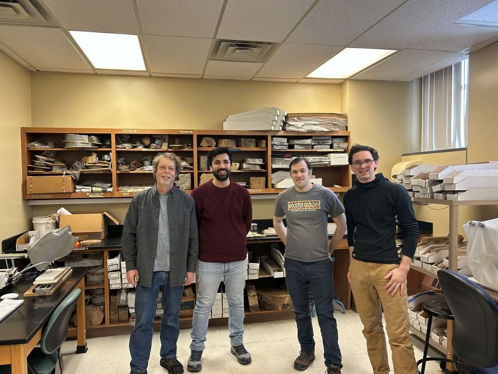
Participants: Greg Wiles, Nick Wiesenberg, Ben Gaglioti, Daniel Mann, Gabrielle Sjoberg, Eloise Peabbles, Eric Benedict, Julian Narvaez, Bob Girt, Arianna Lapke, Lilly Hinkley, Amanda Flory, Michail Protopapadakis, Wenshuo Zhao, Tyrell Cooper, Lynnsey Delio, Isabel Held, Dexter Pakula, Landon Vaughan, Lev Sugerman-Brozan, and AYS students.
General: For the past five years faculty, staff, and students from The College of Wooster Tree Ring Lab, University of Alaska, Fairbanks and the Alaska Youth Stewards (AYS) from Kake, Hoonah, Angoon and Klawock in Southeast Alaska (SEAK) have been collaborating to understand environmental change through the collection of tree-ring data. Together, we sampled and processed eight tree-ring chronologies from a previously under-sampled region of SEAK. These data are records of past climate with direct linkages to cultural and land-use histories. The collection includes the first two western redcedar (Thuja plicata) series for Alaska, one from Kake based on the farthest known north stand of redcedar in its natural range and the other from Klawock. The remaining chronologies include three Alaska yellow cedar (Callitropsis nootkatensis) series from Kake, Hoonah and Klawock, a Sitka spruce (Picea sitchensis) series from Angoon, and two mountain hemlock (Tsuga mertensiana) series from Hoonah and Angoon.
 Background: The collaboration started remotely in the summer of 2021 – the summer of 2022 was a visit to Kake, then Hoonah (2023), Klawock (2024) and then in 2025 Angoon. Throughout the years, all the AYS (Alaska Youth Stewards) groups continued coring trees and sending samples to The Wooster Tree Ring lab and meeting online.
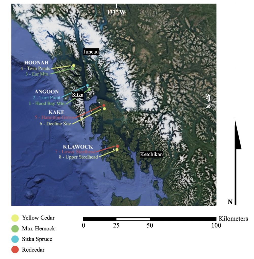
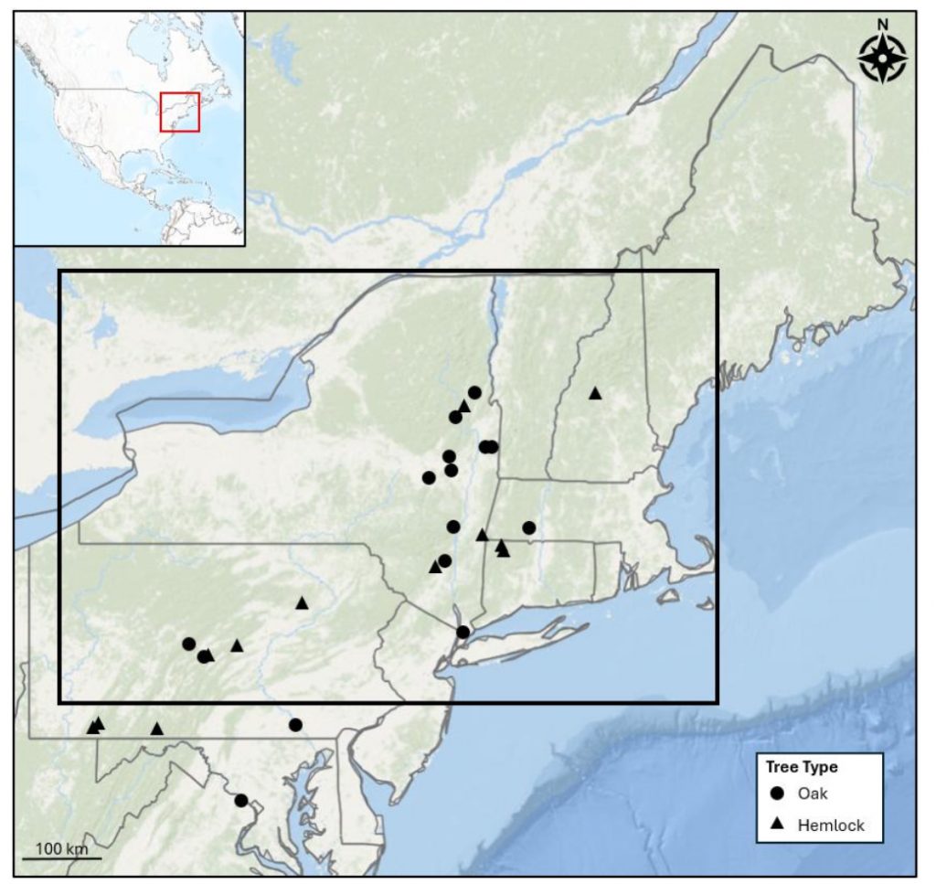
Map showing the location of the eight ring-width sites from Southeast Alaska. Table 1 shows the attributes of each of these chronologies. Note the natural north south transect on which these collections fall.
Table 1. List of the 8 tree-ring sites generated through this collaboration.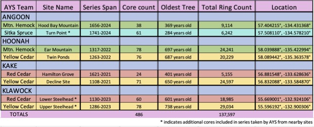
KAKE
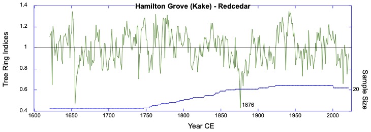
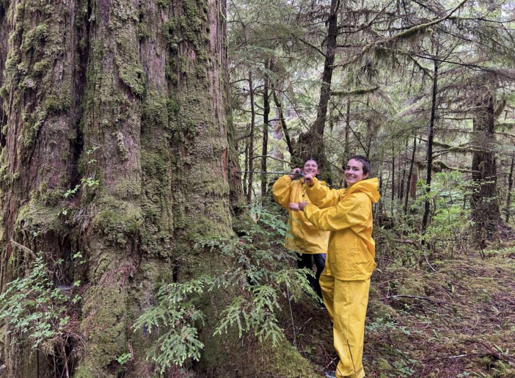
The Hamilton Grove chronology from Kake western redcedar. This redcedar chronology is the first for Alaska and was sampled at the northernmost redcedar site. Other sites further north have been reported, but are not confirmed (pers. comm. B.Buma). The climate signal here is a strong positive relationship with winter temperatures.

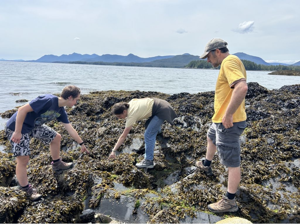
Initial analyses of the red cedar site on a beautiful day on the shores outside of Kake.

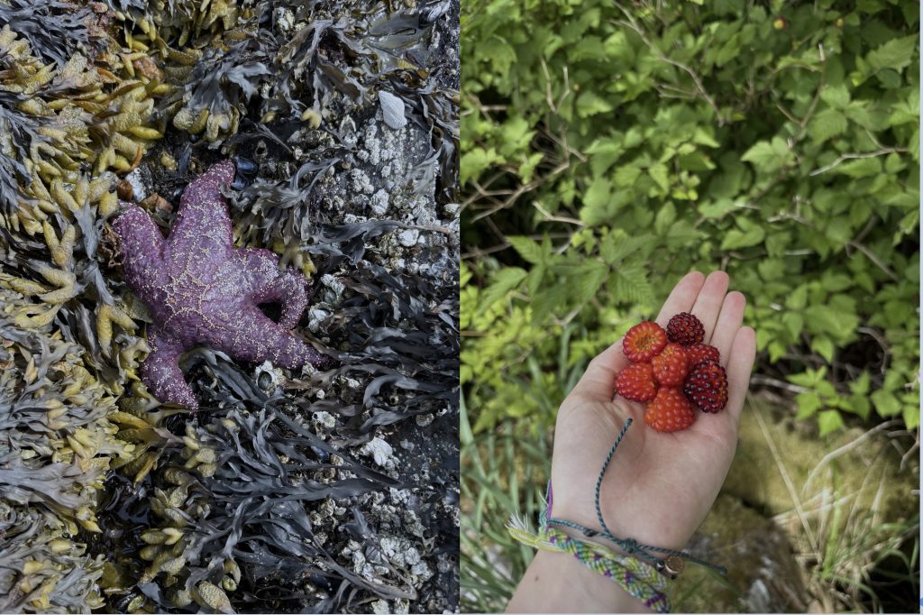
Berry picking was high on the list after the work was done.
HOONAH
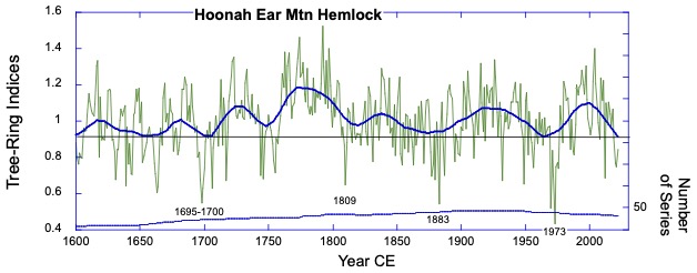
The Hoonah Ear Mountain hemlock site. This site strongly reflects some of the volcanically-forced marker years from the region (late 1690s, 1809, 1883) along with the enigmatic year of 1973, which is a narrow marker year with an uncertain climatic reason.
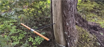 Alaska yellow cedar near Hoonah stripped between 2001 and 2006 CE (Common Era). The year of stripping was determined by coring within and outside of the scar and then taking the difference between the total rings in each core. The stripping is sustainable and not detected as a decline in growth in the ring-width series.

Pickling bull kelp in Hoonah.
KLAWOCK
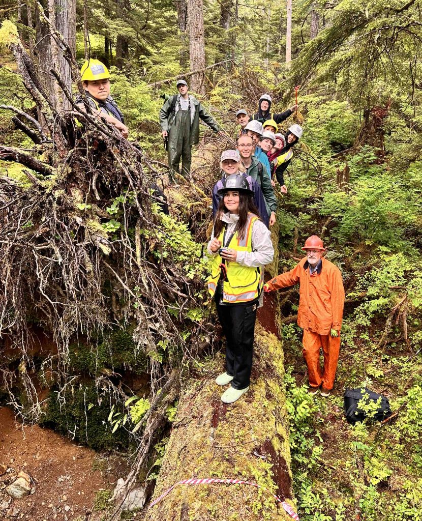
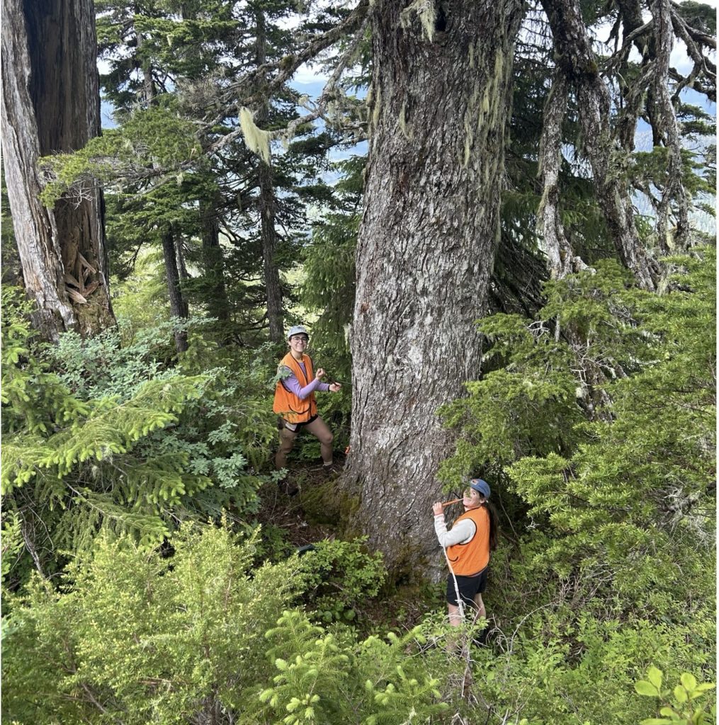
The Klawock-Wooster group in the forest.
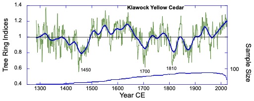
Yellow cedar ring-width series from Klawock – three of the major Northern Hemisphere cooling volcanic eruptions are evident in the record. Comparisons with monthly minimum temperatures from Ketchikan show that March-September correlates most strongly (r = 0.39, p < 0.006, N = 67).

Posing in the yard where yellow and red cedar logs are archived for the artists that will choose these giants for carving canoes and totems.

The group working on yellow cedar cores.
ANGOON
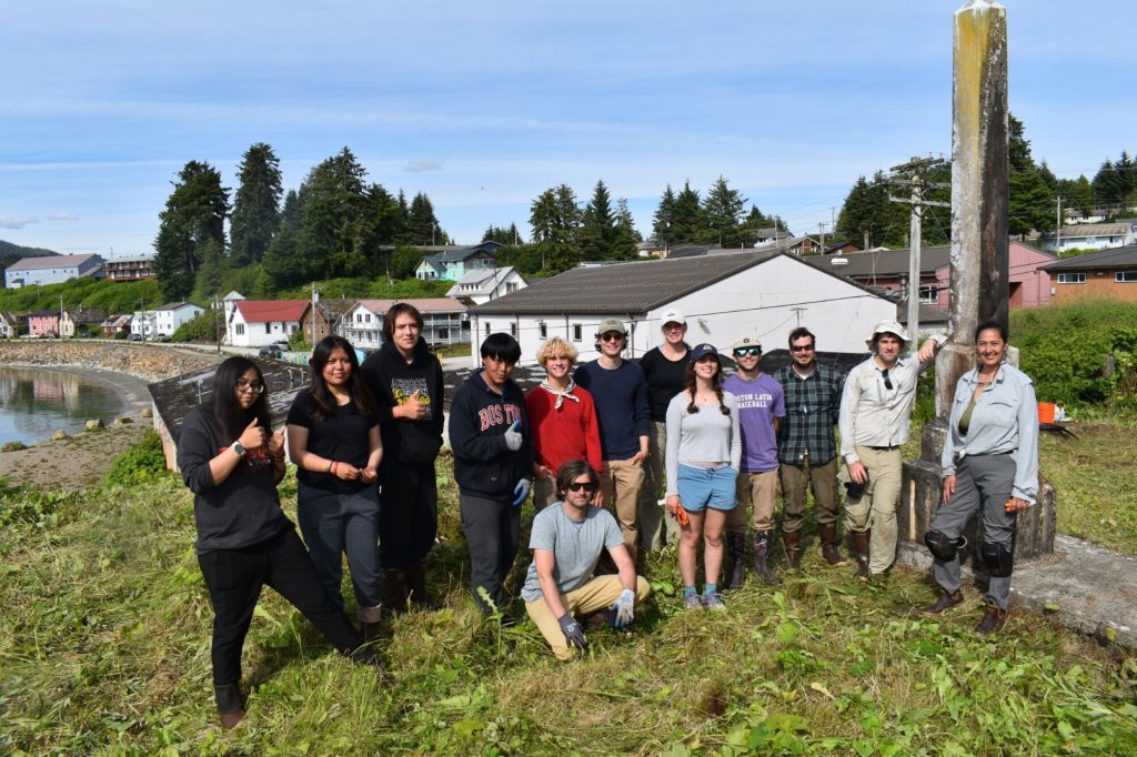
S’eiltin Jamiann Hasselquist (far right) directed the group for a few days of cemetery work in Angoon.
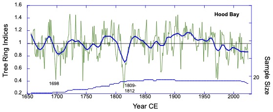
The Hood Bay Mountain, mountain hemlock ring-width chronology. This series is a record of June-August temperatures and shows the volcanic cooling associated with volcanic eruptions at 1698 and 1809. Note also the drop-off after the mid-1970s.
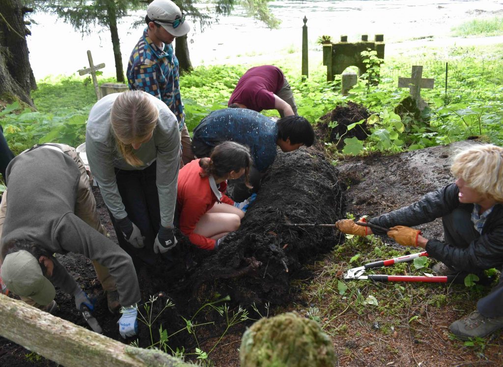
The group peels back the moss and vines to reveal another Tlingit grave.
Acknowledgements: This work was supported by the National Science Foundation under grants P2C2-2002561and P2C2-2002454, and through the Keck Geology Consortium NSF grant 2050697. We also thank The College of Wooster Danner Fund.

Wooster participants on the first trip to Kake.
References (the tree-ring data are available using the links below):
Wiles, G.; Wiesenberg, N., 2026. Turn Point Update – PISI – ITRDB AK213, https://www.ncei.noaa.gov/access/paleo-search/study/44480https://doi.org/10.25921/tc7z-cf17
Wiles, G.; Wiesenberg, N.; Zhao, W.; Hinkley, L., 2026. Hamilton Grove – THPL – ITRDB AK216, https://www.ncei.noaa.gov/access/paleo-search/study/44483, https://doi.org/10.25921/rsgt-1519
Wiles, G.; Wiesenberg, N.; Flory, A.; Protopapadakis, M., 2026. Klawock Redcedar Comp – THPL – ITRDB AK217, https://www.ncei.noaa.gov/access/paleo-search/study/44484, https://doi.org/10.25921/ekbp-3m14
Wiles, G.; Wiesenberg, N.; Flory, A.; Protopapadakis, M., 2026. Klawock Yellow Cedar Comp – CHNO – ITRDB AK218, https://www.ncei.noaa.gov/access/paleo-search/study/44485, https://doi.org/10.25921/4k9k-1c63
Wiles, G.; Wiesenberg, N.; Cooper, T.F.; Gaglioti, B.V.; Hinkley, L., 2026. Hoonah Yellow Cedar – CHNO – ITRDB AK219, https://www.ncei.noaa.gov/access/paleo-search/study/44486, https://doi.org/10.25921/4bhp-1b59
Wiles, G.; Wiesenberg, N.; Cooper, T.F.; Gaglioti, B.V.; Hinkley, L., 2026. Hoonah Ear Mountain – TSME – ITRDB AK222, https://www.ncei.noaa.gov/access/paleo-search/study/44489, https://doi.org/10.25921/9pwx-mc46
Wiles, G.; Wiesenberg, N., 2026. Hood Bay Mountain – TSME – ITRDB AK223, https://www.ncei.noaa.gov/access/paleo-search/study/44490, https://doi.org/10.25921/mr27-g619


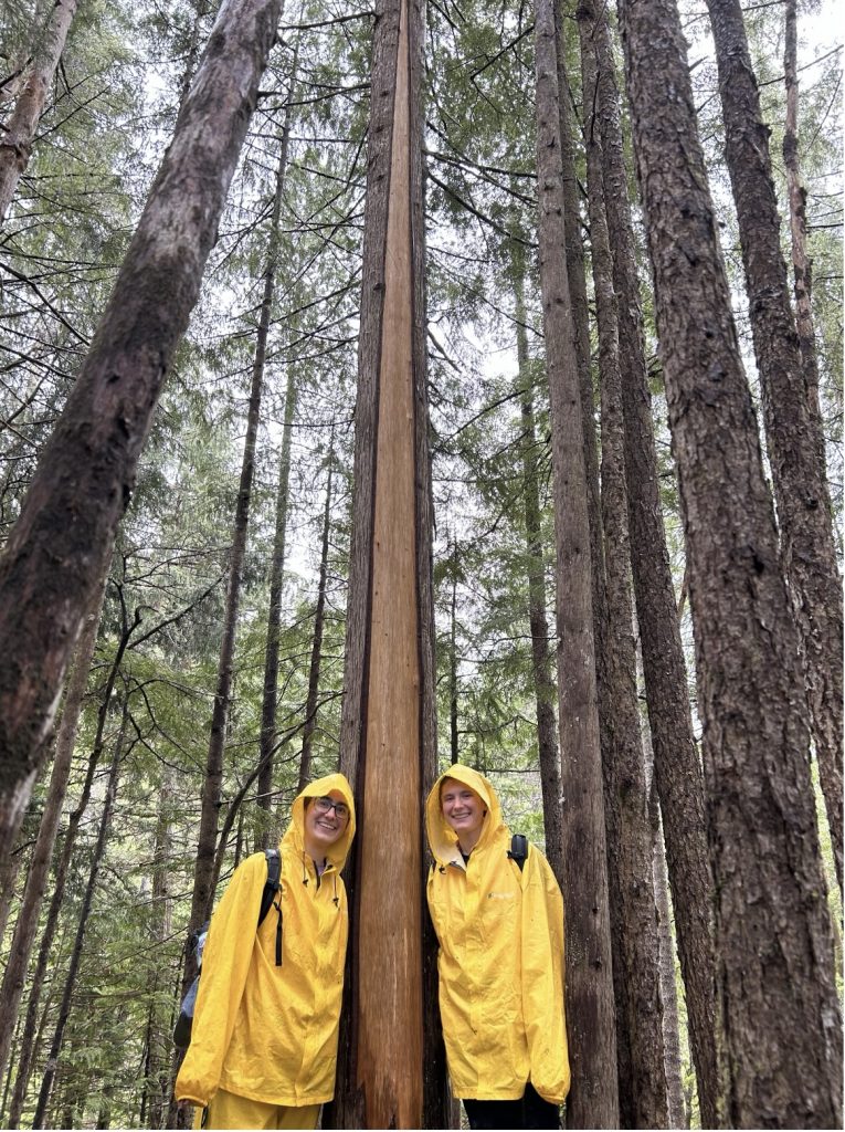
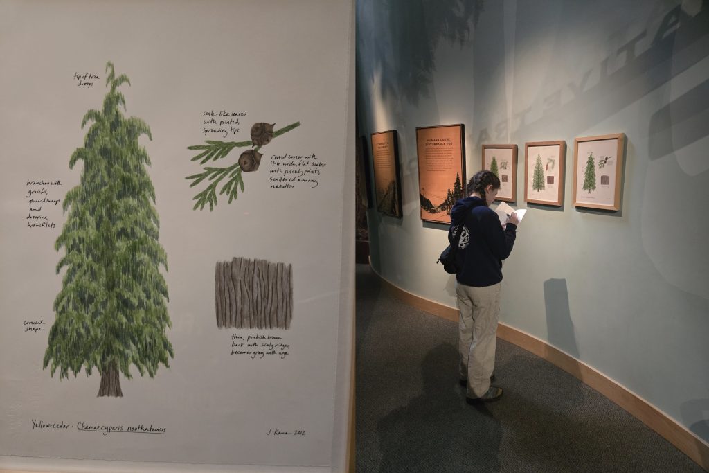
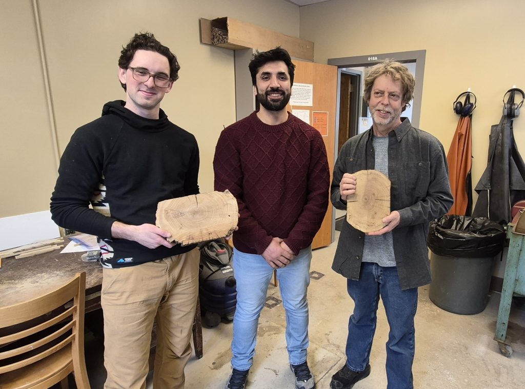
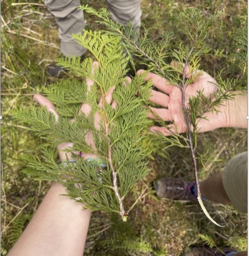 Yellow cedar (left) and redcedar (right)
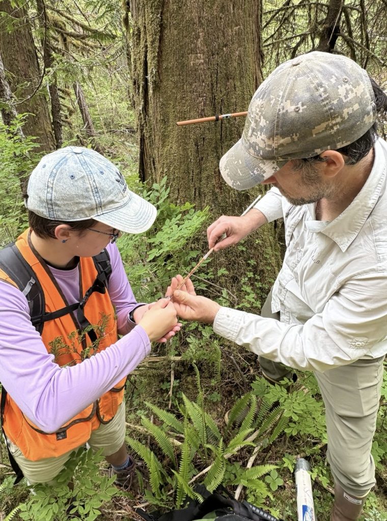
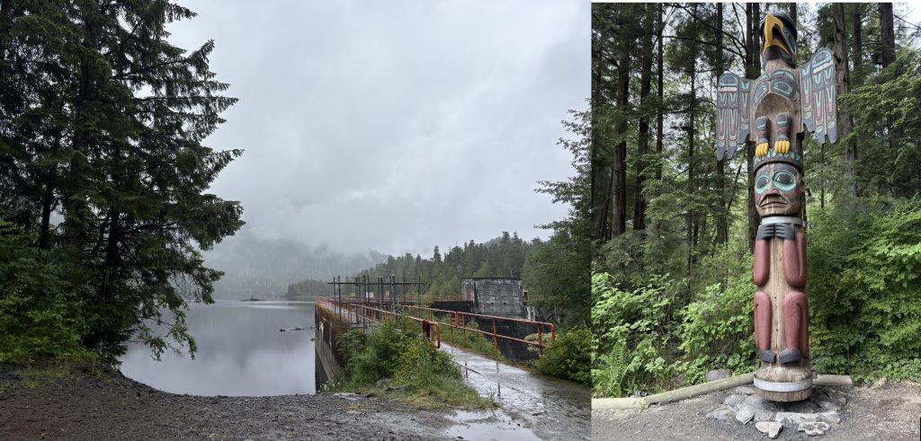
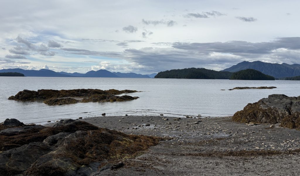
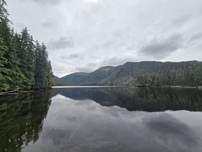 Perseverance Lake.