There’s two weeks left in the semester, so today on Climate Monday we’re going to take things to the next level and highlight not only visualization, but also analysis of climate data. Most of the big papers in climatology nowadays involve more data than you can shake a stick, and they require so computer science chops to make happen. However, if you’re in the exploration phase, going through all that coding can be excessive work and it’s better to have a quick-and-dirty tool to get a sense of what’s going on. The tool my PhD advisor always uses is the NCEP/NCAR reanalysis compositor. “NCEP” is the National Center for Environmental Prediction and “NCAR” is the National Center for Atmospheric Research. But what is a “reanalysis”?
What is a Reanalysis?
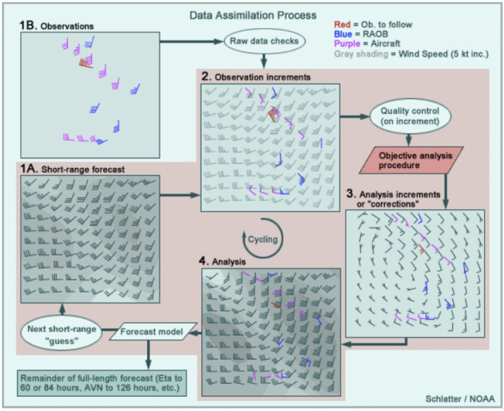
Figure 1: How to create an atmospheric “analysis”. Credit: NOAA
Well, to start we have to define an atmospheric “analysis”. And to do that, we actually need to start with an atmospheric weather “forecast”. Whew. A weather forecast might be familiar; it’s an assessment of what atmospheric conditions are likely to be sometime in the future. Today, our weather forecasts are derived from weather models. We may like to joke about how bad they are, but for predicting the weather an hour from now, weather models are extremely accurate throughout most the US (especially in flatter areas like Ohio). However, these models are not perfect, and the analysis process accounts for that. To make an analysis, you also need to gather a bunch of atmospheric observations. These can be from a variety of sources, like aircraft, ships, land-based stations, weather balloons, or satellites. If you take, for example, the wind forecast for 6 AM that was made back at 5 AM (i.e., the 1-hr forecast — Step 1A in Figure 1) and then compare it to observations (Step 1B), you’ll find that they don’t line up perfectly (Step 2). The “analysis” step is to alter the 1-hr forecast so that it more closely matches the observations (Step 3). The best solution usually is not to make the forecast perfectly match observation points, because observations have error too. Indeed, the model is often more accurate in places that are remote (e.g., the Arctic Ocean) or notoriously “noisy” for data collection (e.g., Mount Elbert in Colorado). The result of this assimilation process is the “analysis” (Step 4). This analysis then becomes the input for the next 1-hr run of the weather model.
The difference between an “analysis” and a “reanalysis” is that the former is operational while the latter is academic. In practice, weather forecasters are constantly tweaking their models to improve forecasting, but that can lead to weird biases in long-term data; model output from 1980 is not directly comparable to model output from 2015. So with a “reanalysis”, researchers decide on a single model set-up and re-run everything. That’s right: for every hour, they re-run the model, re-run the assimilation of observations, and spit out an analysis. This is what the NCEP/NCAR reanalysis tool is, and it’s a great way to start thinking about climate analysis instead of just weather analysis.
Examples from NCEP/NCAR Reanalysis
We’ll stick to surface temperature, because that’s a pretty simple variable to talk about, but note that you can look at a whole suite of variables from multiple levels in the atmosphere. It’s not very detailed information — you can’t use this tool to think about individual cities — but for a broad view, you can see, for example, that average temperatures in the US in March ranged from sub-freezing in Minnesota to over 20°C (68°F) in southern Florida. Note, it’s much worse up in Hudson Bay, where temperatures averaged about -15°C (5°F). (Figure 2)
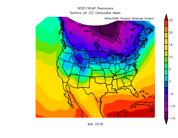
Figure 2: Average surface air temperature in Mar 2018 compared to 1981-2010 average. Source: NCEP/NCAR Reanalysis
You can also check out how March 2018 compared to “normal” (meaning the average from 1981 to 2010). As noted a few weeks ago on this blog, northeast Ohio and Virginia and eastern Montana were all cooler than average by a few degrees. Of course, Texas was a little bit warmer than average. (Figure 3)
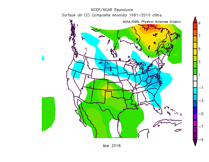
Figure 3: Surface air temperature anomaly in Mar 2018 compared to 1981-2010 average. Source: NCEP/NCAR Reanalysis
That’s good, but you can see all of this at NOAA’s website, too for the past month with fewer clicks. So what makes the NCEP/NCAR compositor special is the ability to composite random years together and keep experimenting until the cows come home. For example, did you know that in the autumns (Sep, Oct, Nov) with presidential elections, years in which the USA elects a Democrat tend to be cooler in the East and warmer in the West? (Figure 4). Now, I don’t think that’s a significant result, and I doubt it really means anything. On the other hand, knowing politics, don’t be surprised if you start seeing Republicans with hair dryers in Michigan come October 2020.
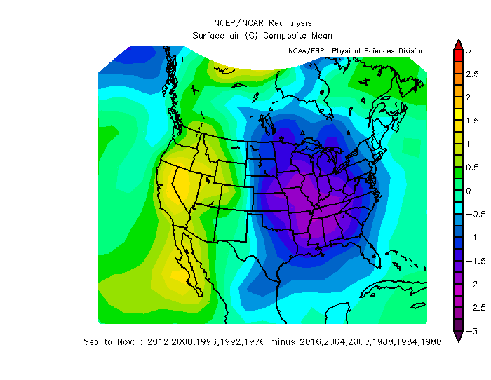
Figure 4: Difference in Sep-Nov surface air temperature between years in which a Democrat won the presidential election in the US minus years in which a Republican won. Source: NCEP/NCAR Reanalysis.


 Santa Clara, Utah — Visiting Zion National Park is an obvious activity for Team Jurassic Utah, considering it is made of beautiful Jurassic rocks. We took the opportunity today. Well, half of the team. Galen and I weren’t feeling well, so Nick took Ethan to the magnificent place. Here they are at The Narrows, with some random people above watching. They had a great time as Galen and I recovered quickly enough back at the base.
 Speaking of our base, I should describe it. Our place in Santa Clara is embarrassingly luxurious. I’m forbidden from camping out in southern Utah (an incident with gnat bites and anaphylaxis about 20 years ago!), so I usually stay in motels. Our administrative coordinator Patrice Reeder had a great idea: why not look into Airbnb rentals in the area? She found one on our main route to Gunlock. It is indicated by the red pin above near the southern end of the Santa Clara lava field. Appropriately, this place is called Lava Falls at Entrada. It is significantly cheaper than motel rooms, and much more roomy and private. We’ve also saved on food as Nick, Galen and Ethan are avid (and skilled) cooks.
 Here is our own Lava Falls #8 house. The attached garage makes it even more convenient for storing gear and specimens, and for loading and unloading the vehicle.
 As you saw from the aerial image, this development is in the lava field, remnants of which surround us. For geologists, this has been a very convenient, comfortable and efficient place to stay. Great idea, Patrice.
 Nick brought his mountain bike on the trip, which has been highly useful in the field because he can go off on scouting trips and cover a lot of territory. He also likes to ride the trails at night because of the cool air and lack of other people. Last night he met up with a fox and got this great picture.