Washington, Utah — In March 2020 a team of Wooster Geologists was in beautiful southwestern Utah sampling, measuring and analyzing rocks and fossils from the Middle Jurassic Carmel Formation north of St. George. The Covid-19 pandemic forced us to end that trip and retreat to Wooster. Surely, we thought, at the very least we will be able to return in the summer, but you know that story. Finally, after 26 months, a new team is back on those fascinating rocks.
Pictured above in the now-classic scene is Team Jurassic Utah 2022 posing in front of the Carmel Formation exposed on the northern shore of Gunlock Reservoir. On the left is Nick Wiesenberg, our indispensable geological technician. To the right are then Shipei (Vicky) Wang (’23), Lucie Fiala (’23), and Professor Shelley Judge. It is a beautiful May day as we begin our geological orientation. The primary goal of this expedition is to collect specimens, measurements and observations to support the Senior Independent Study projects of Vicky and Lucie.
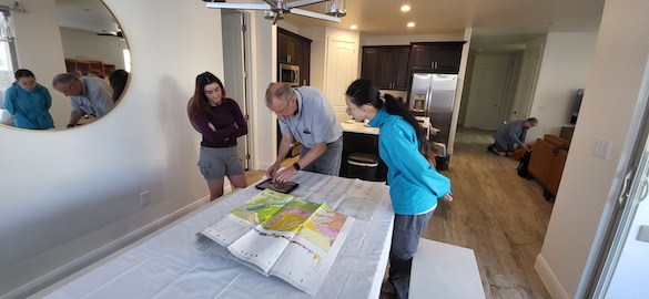 We are fortunate geologists indeed to be able to stay in an Air BnB house in Washington, Utah, during our fieldwork. This morning we started with a briefing about the day’s activities. (Lucie on the left, Vicky on the right.) Note the geological map and stratigraphic sections supplemented by an iPad. (Photo by Nick.)
 Our first field task was to find an outcrop for Lucie’s Senior IS project. She is looking at the Co-Op Creek Limestone Member of the Carmel Formation, concentrating on the transition between the informal “lower” portion and the informal “upper” part. This corresponds with the boundary between the (again informal) C and D members of Nielson (1990). The lower member is a distinctive set of supratidal and intertidal facies dominated by stromatolites, some of which were examined by Will Santella (’21) in his Senior IS. We found a nice exposure of these stromatolites just northeast of the Gunlock Reservoir.
 Some of these stromatolitic and microbial mat deposits have remarkable burrows filled by a well-sorted calacreous sand that appears to be made mostly of crinoid debris.
 Lucie and Vicky examine one of the stromatolite beds.
 These lower Carmel Formation units also include well-preserved current ripple marks.
 Here we are having lunch at one of our most interesting outcrops so far. These almost white rocks weather very differently than the usual limestones and shales above and below them. Turns out this is an exposure of the lowest rocks of the upper part of the Co-Op Creek Limestone Member. (Photo by Nick.)
 This white unit is a sandstone at N 37.282454°, W 113.803273°. We have a hypothesis that the lower-upper transition here marks a Middle Jurassic transgression (when sea level rises relative to the land). Sandstone is very rare in the Carmel Formation, so it is telling us something significant about the transition from intertidal to subtidal environments. Score one important find for our first day.
 Lucie demonstrates above how unconsolidated this sand is in places. We can run this sand through our venerable Ro-Tap!
 The units immediately above the white sandstone include the familiar ooid shoal deposits of the upper part of the Co-Op Creek Limestone Member. These were studied by Anna Cooke (’20) in her Senior IS project.
 A closer view of the ooid shoal deposits and underlying shales.
We will return to these outcrops tomorrow for full measurement, description and sampling.
 Nick photographed this blooming prickly pear cactus near our study site today.
 And Nick encountered our first rattlesnake of the season! This scary beauty is a Western Diamondback Rattlesnake. I hope it is the last one we see!
 The head of this snake with its creepy tongue deserves a close-up!
References: (Which will be useful later.)
Nielson, D.R. 1990. Stratigraphy and sedimentology of the Middle Jurassic Carmel Formation in the Gunlock area, Washington County, Utah. Brigham Young University Geology Studies 36: 153-192.
Sprinkel, D.A., Doelling, H.H., Kowallis, B.J., Waanders, G., and Kuehne, P.A., 2011, Early results of a study of Middle Jurassic strata in the Sevier fold and thrust belt, Utah, in Sprinkel, D.A., Yonkee, W.A., and Chidsey, T.C., Jr., eds., Sevier thrust belt: northern and central Utah and adjacent areas: Utah Geological Association Publication 40, p. 151-172.
Taylor, P.D. and Wilson, M.A. 1999. Middle Jurassic bryozoans from the Carmel Formation of southwestern Utah. Journal of Paleontology 73: 816–830.
Wilson, M.A. 1998. Succession in a Jurassic marine cavity community and the evolution of cryptic marine faunas. Geology 26: 379–381.
Wilson, M.A. 1997. Trace fossils, hardgrounds and ostreoliths in the Carmel Formation (Middle Jurassic) of southwestern Utah, in Link, P. and Kowallis, B., eds., Mesozoic to recent geology of Utah, Brigham Young University, v. 42, p. 6–9.
Wilson, M.A., Ozanne, C.R. and Palmer, T.J. 1998. Origin and paleoecology of free-rolling oyster accumulations (ostreoliths) in the Middle Jurassic of southwestern Utah, USA. Palaios 13: 70–78.


 This morning the Wooster Geologists visited the westernmost exposure of the lower Carmel Formation at Nielson’s (1990) Jackson Peak section. Nick and Vicky are shown above on the road towards the conical Jackson Peak in the background. The site was as buggy as any other on this trip, with not a breath of wind to relieve us.
 Nick took this image of our team hiking up a wadi in search of a good place to make a stratigraphic column. Jackson Peak looms in the background.
 We established the base of the section in a wadi at N 37.327356°, W 113.858144°. Because of the rough terrain, the gnats, and the mostly-covered nature of the stratigraphy here, we decided to use Nielson’s (1990) original measurements and then sample along his column. Note that burned trees give very little shade.
 Another image by Nick of Wooster Geologists at work. In the background is Square Top Mountain, which is most notable as the site of a B-52G crash in 1983.
 This is the highest in-place outcropping of the typical lower Carmel Formation stromatolitic micrite beds. You can see the fine microbial layering on the weathered surfaces of the rock. Sampled as JP-1.
 Like an old friend, the distinctive sandstone we saw in the Manganese Wash section showed up here at Jackson Peak. It has the same weathering appearance and, at the handlens level, the same lithological composition. Sampled as JP-2.
 Unlike at the Manganese Wash section, the sandstone at Jackson Peak has an ooid shoal biosparite/grainstone directly above it, our sample JP-3.
 This ooid shoal deposit as the same low-angle cross-bedding and current ripple marks as we’ve seen in all our Carmel Formation sections.
 At the top of the ridge we were studying, Lucie and Vicky came across our second rattlesnake of the trip. It buzzed immediately, so Lucie and Vicky moved away quickly. Nick got this great image.
 On our way back from the Jackson Peak section we met two Bureau of Land Management officers on horseback. Now there’s a cool job. (Photo by Nick.)
 As is our tradition on these southwestern Utah expeditions, after we finished our work at Jackson Peak, we visited the 1857 Mountain Meadows Massacre site a few miles to the north.
 This is the cairn marking the mass grave of 34 of the victims buried on the massacre site. It is a sad and enraging story we encourage you to read at the link above.