New York, NY – [Guest Blogger Annette Hilton]
This summer I have the privilege of working and living in New York City at the American Museum of Natural History. I, along with several other students, have the opportunity to work with the museum’s researchers through an REU (Research Experience for Undergraduates) program funded by the National Science Foundation.
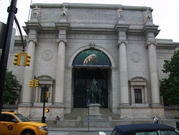
Front entrance of the American Museum of Natural History (AMNH).
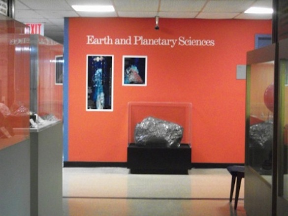
Entrance to the Earth and Planetary Sciences Department, AMNH.
As a geologist, I am working in the Earth and Planetary Sciences Department. I am under the mentorship of Dr. Juliane Gross, a research associate at the museum. Together we have been working with a small sample from an unnamed lunar meteorite found in Northwest Africa. Our goal for the end of the summer is to classify and name this mysterious lunar meteorite.
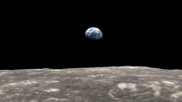
Photo from: http://www.nasa.gov/sites/default/files/moon_and_earth_lroearthrise_frame_0.jpg
Meteorites are undoubtedly cool, but why should we care so much about the Moon? According to the Giant Impact Hypothesis, around 4.5 Ga proto Earth collided with another planetary body called Theia. Though an extremely violent impact, Earth quickly reformed and the remaining debris circled our planet, eventually forming the Moon. This theory is generally accepted but still under reform. We know that the Moon and Earth are extremely similar in composition, making their dual formation likely.
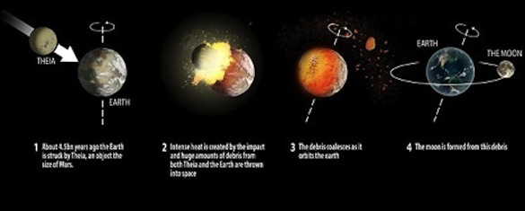
What the formation of Earth and the Moon may have looked like.
Photo from: http://www.dailymail.co.uk/sciencetech/article-2650130/How-moon-formed-Researchers-reveal-new-evidence-Earth-hit-giant-object-4-5-billion-years-ago.html
Because the Moon and Earth are so similar, we can study the Moon to gain information about our early solar system and early Earth. If we want to know more about how Earth formed, how old it is, and what the proto-material was like, we can turn to our closest neighbor in the solar system. Because the Moon is no longer geologically active, it has preserved information from the span of over 4.0 Ga. This is a sharp contrast to Earth, whose original material has all since been recycled.
Before the Apollo and Luna missions, lunar information was all theory. We had no data to put lunar theories into context and were unable to classify lunar meteorites because we had nothing to compare them to. From all of the Apollo missions, only ~382 kg of lunar rocks and soils were brought back. Because of logistical reasons, all of the lunar missions landed and collected samples in the same relatively small area: the lunar mare.
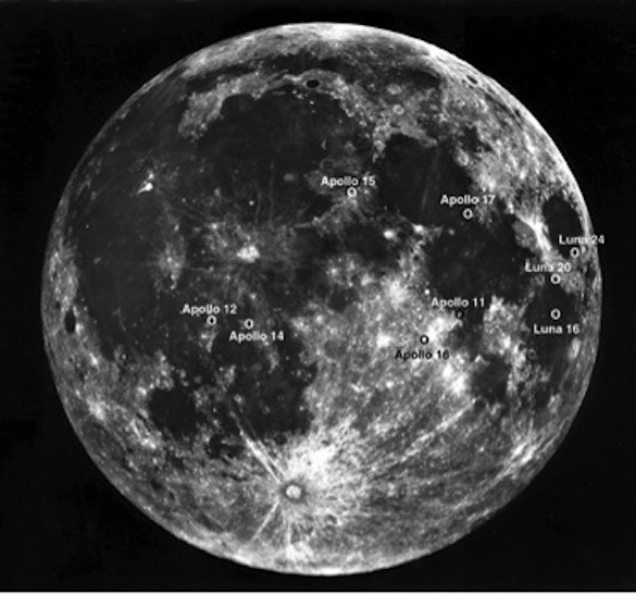
Mapped image of the Moon with Apollo and Luna missions landing sites.
Photo from: http://www.lpi.usra.edu/science/kring/epo_web/moon/moon_image7.jpg
Later, data collected by satellites would show this area to be a chemical anomaly in comparison to the rest of the Moon. The lunar mare largely contains higher levels of elements including rare earth elements (REEs) in comparison to the rest of the Moon.
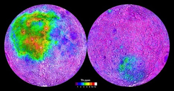
Elemental map of the Moon showing high levels of Thorium in areas of Apollo and Luna landings.
Photo from: https://upload.wikimedia.org/wikipedia/commons/9/93/Lunar_Thorium_concentrations.jpg
So now we know that the samples collected from the Moon aren’t representative of its entire body. Much of what we consider to know and understand about the Moon today were based on Apollo, Luna samples and information. Because these samples aren’t representative, it is necessary to take a critical look at our current understanding of the Moon. Until we return, our only source of lunar rocks that come from places other than where the Apollo/Luna samples were collected are meteorites. So if we want to gain a clearer understanding of what the Moon is really like, we must study them.
You may be wondering how lunar meteorites arrive on Earth in the first place. Lunar meteorites come from the ejecta during an impact event on the Moon. When a meteoroid or other asteroidal body hits the Moon’s surface, lunar crust is displaced and gets ejected into space, eventually becoming trapped in Earth’s gravity field, allowing it to come to our surface.
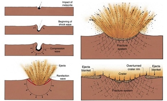
Diagram of a meteoroid impact.
Photo from: http://explanet.info/images/Ch04/04_03.jpg
Meteorites are usually collected in deserts, like the Sahara or Antarctica, because they are easily located and preserved well in these areas. Teams of scientists search for meteorites each year in key locations and may at best return with some hundreds of samples.
Among those, only a small fraction may be lunar. On the whole, lunar meteorites are very rare–there have only been a total of 110 total unpaired lunar meteorites ever found.
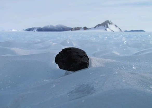
Image of meteorite, exhibiting fusion crust, in Antarctica.
Photo from: https://earthandsolarsystem.wordpress.com/2013/01/21/ansmet-meteorite-hunting-2012-2013-season-draws-to-an-close/
Even though samples are limited, each new lunar meteorite gives us another chance to learn more about the Moon and expand our understanding of it.
In order to learn about our meteorite, my advisor and I have been studying our sample through chemical analysis and elemental x-ray mapping, which is done with an Electron Probe Micro-Analysis (EPMA). The machine can be programed to map the element distribution of the entire sample or just specific areas, but depending on the size of the area to be mapped the analysis can take several days. By analyzing single minerals within the sample we can get mineral chemistry in oxide weight percent, which has helped us to understand the mineralogy and petrography of our sample.
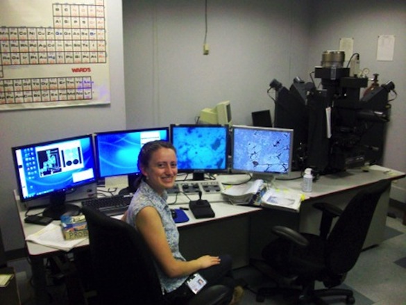
Annette Hilton (‘17) programing analysis of the unknown lunar meteorite in the EPMA, located in the Earth and Planetary Sciences Department at AMNH.
Soon we will be conducting LA-ICP-MS (laser ablation inductively coupled plasma mass spectrometry) on the sample to get data on trace and REEs that might be in our meteorite but are too minute for the EPMA to detect. This finer analysis will allow us to compare our sample more comprehensively to other lunar samples, and perhaps even hypothesize crystallization history. Currently we are working to calculate the bulk composition of our sample, which would enable us to use whole rock analysis as another comparative tool. Looking forward, we also hope to use the presence of different pyroxenes in the sample to calculate crystallization temperature, which could help us further understand our sample’s formation history.
By the end of the summer at AMNH we hope to submit a classification for the meteorite and work to publish about the sample. I am incredibly grateful for this exciting and valuable opportunity to learn and contribute towards lunar work.
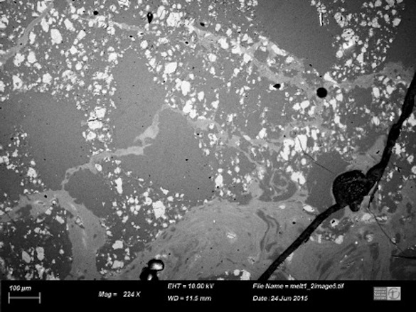
SEM (Scanning Electron Microscope) image of our unknown lunar sample. Shown above is a terrestrial alteration crack, several melt veins (from shock impact), and plagioclase grains outlined by a matrix of olivine and pyroxene grains.
Thank you to AMNH, NSF REU Program for Physical Sciences, Dr. Juliane Gross, and of course our wonderful professors at Wooster (particularly Dr. Meagen Pollock, professor of Mineralogy and Petrology).
References:
Gross, J., Treiman, A.H., and Mercer, C.N., 2014, Lunar feldspathic meteorites: constraints on the geology of the lunar highlands, and the origin of the lunar crust: Earth and Planetary Science Letters, v. 388, p. 318–328.
Joy, K.H., and Arai, T., 2013, Lunar meteorites: new insights into the geological history of the Moon: Astronomy & Geophysics, v. 54, p. 4–28.
Korotev, R.L., 2005, Lunar geochemistry as told by lunar meteorites: Chemie der Erde-Geochemistry, v. 65, p. 297–346.
Taylor, S.R., Taylor, G.J., and Taylor, L.A., 2006, The moon: a Taylor perspective: Geochimica et Cosmochimica Acta, v. 70, p. 5904–5918.
Treiman, A.H., Maloy, A.K., Shearer, C.K., and Gross, J., 2010, Magnesian anorthositic granulites in lunar meteorites Allan Hills A81005 and Dhofar 309: Geochemistry and global significance: Meteoritics & Planetary Science, v. 45, p. 163–180.